基于物理的着色理论¶

材质（Material）描述的是光到物体表面后如何被反射，就是渲染方程中的 BRDF。

Diffuse / Lambertian BRDF¶

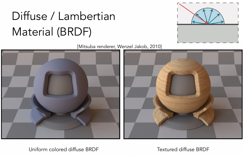
光会均匀地被反射到各个方向。假设各个方向的入射光也是一样的，那么 \(f_r(\omega_i,\omega_o)\)、\(L_i(\omega_i)\) 和 \(L_o(\omega_o)\) 都是常量

\[ \begin{align} L_o(\omega_o)&=\int_{H^2} f_r L_i \cos \theta_i \mathrm{d}\omega_i\\ \\ &=f_r L_i \int_{H^2} \cos \theta_i \mathrm{d}\omega_i\\ \\ &=\pi f_r L_i \end{align} \]

其中 \(H^2\) 是法线方向的半球。如果表面的反照率（Albedo/Color）是 \(\rho\)，那么有 \(L_o=\rho L_i\)，所以

\[ f_r=\frac{\rho}{\pi} \]

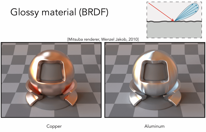
Glossy BRDF¶

Ideal Reflective / Refractive BSDF¶

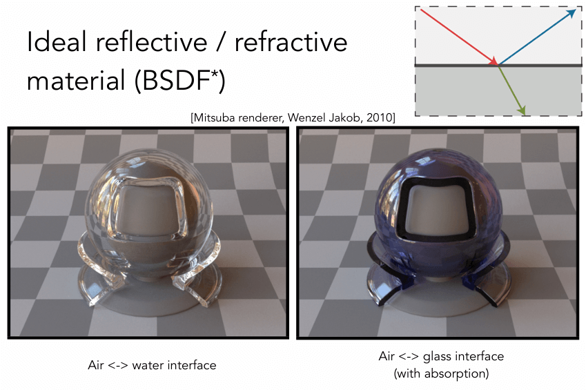
光会发生反射和折射。使用 BRDF 描述反射，BTDF (Bidirectional Transmittance Distribution Function) 描述折射，两个加起来称为 BSDF (Bidirectional Scattering Distribution Function)，即 BSDF = BRDF + BTDF。

Perfect Specular Reflection¶

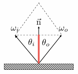
反射角等于入射角 \(\theta_o=\theta_i=\theta\)

\[ \omega_o+\omega_i=2 \cos \theta \ \vec{n} = 2 (\omega_i \cdot \vec{n})\vec{n} \]

所以

\[ \omega_o=-\omega_i + 2 (\omega_i \cdot \vec{n})\vec{n} \]

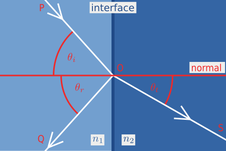
Snell's Law¶

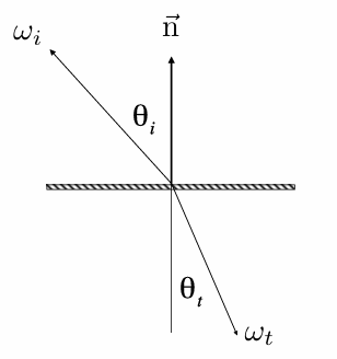
入射角 \(\theta_i\) 和折射角 \(\theta_t\) 满足

\[ \eta_i \sin \theta_i = \eta_t \sin \theta_t \]

其中 \(\eta_i,\eta_t\) 是两种介质的折射率（Index of Refraction / IOR）。

\[ \cos \theta_t = \sqrt{1 - \left(\frac{\eta_i}{\eta_t} \right)^2 (1-\cos^2 \theta_i)} \]

当 \(\dfrac{\eta_i}{\eta_t}>1\) 时，如果 \(\theta_i\) 足够大，上式根号里的部分就会小于 0，所以当光从光密介质进入光疏介质，且入射角足够大时，会发生全反射（Total Internal Reflection）。

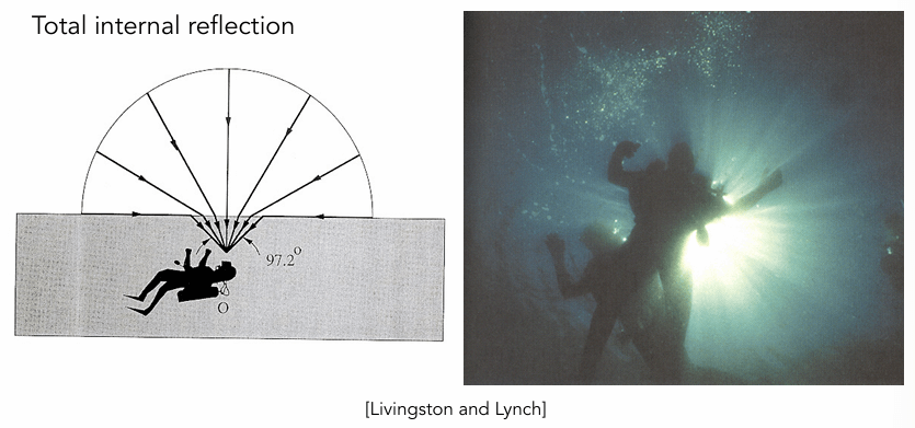
从水底往上看，只有 97.2 度锥形范围的光来自天空，剩下的来自水下的光在水面的全反射。

Fresnel Reflection / Term¶

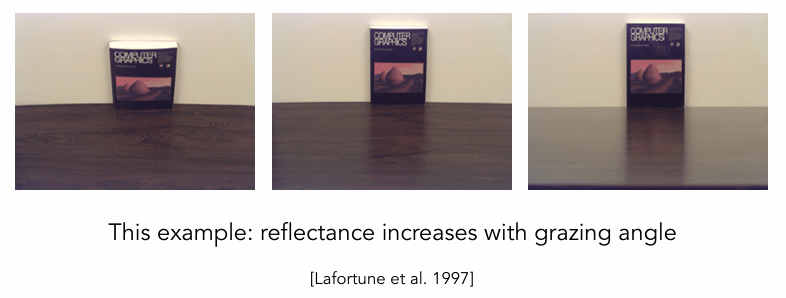
Reflectance depends on incident angle (and polarization of light)

反射现象和光的入射角以及偏振有关，入射角越大，反射越强。又因为反射角等于入射角，所以视线越靠近表面，看到的反射越强。

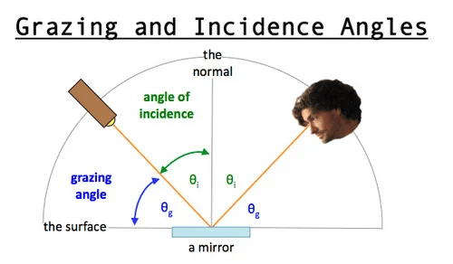
Grazing Angle

掠射角（Grazing Angle）指的是与入射角互余的角，即光与表面切线的夹角。另一方面，当入射角接近 90 度时，称为「掠射」，所以很多时候掠射角仅表示入射光非常接近表面的时候。

"Graze" and "grazing" in English refer to animals eating grass close to the ground, and from that, "to graze" can also mean "to touch lightly the surface of an object in passing."

Describing an angle between two objects moving past each other as "grazing" would imply that the angle is small because they almost touched.

So in graphics, the "90-degree complement to the angle of incidence" is generally only referred to as a "grazing angle" when, like you said, the angle of the light traveling above the surface is very small, almost parallel to that surface. ¹

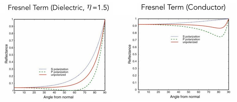
给定入射角 \(\theta_i\)，Fresnel Term 给出了对应的反射率。上图中，左边是绝缘体（Dielectric），右边是导体（Conductor）。

\[ \begin{align} R_s &= \left|\frac{n_1 \cos \theta_i - n_2 \cos \theta_t}{n_1 \cos \theta_i + n_2 \cos \theta_t} \right|^2 = \left|\frac{n_1 \cos \theta_i - n_2 \sqrt{1-\left(\dfrac{n_1}{n_2} \sin \theta_i\right)^2}}{n_1 \cos \theta_i + n_2 \sqrt{1-\left(\dfrac{n_1}{n_2} \sin \theta_i\right)^2}} \right|^2\\ \\ R_p &= \left|\frac{n_1 \cos \theta_t - n_2 \cos \theta_i}{n_1 \cos \theta_t + n_2 \cos \theta_i} \right|^2 = \left|\frac{n_1 \sqrt{1-\left(\dfrac{n_1}{n_2} \sin \theta_i\right)^2} - n_2 \cos \theta_i}{n_1 \sqrt{1-\left(\dfrac{n_1}{n_2} \sin \theta_i\right)^2} + n_2 \cos \theta_i} \right|^2\\ \end{align} \]

通常不考虑偏振（含有等量的 s 偏振和 p 偏振），那么反射比为

\[ R=\frac{1}{2}(R_s+R_p) \]

这个公式太复杂，所以常用 Schlick's approximation²

\[ R(\theta)=R_0+(1-R_0)(1-\cos \theta)^5 \]

随着入射角 \(\theta\) 变大，\(R(\theta)\) 从初始值 \(R_0\) 增大到 \(1\)。其中

\[ R_0=\left(\frac{n_1-n_2}{n_1+n_2}\right)^2 \]

Microfacet Theory¶

物体表面由很多微表面组成，每个微表面都是平坦的，且有自己的法线。通常把每个微表面都当成一个完美的菲涅尔镜面，也可以根据需要选择其他做法。

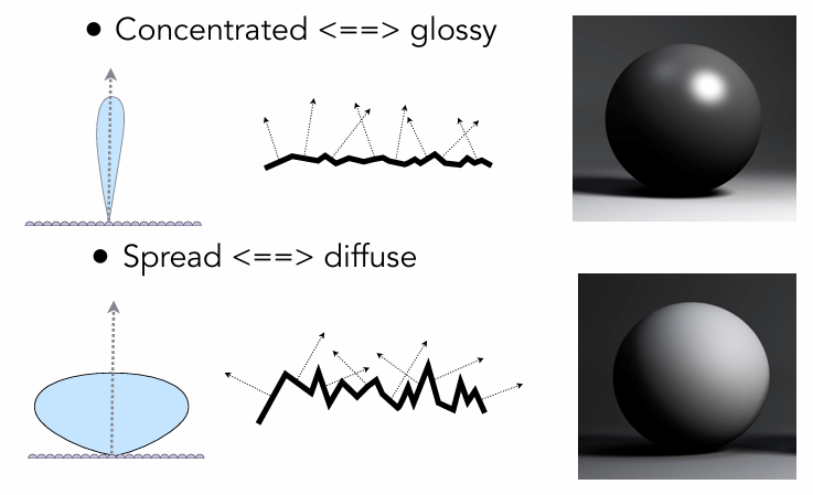
Key: The Distribution of Microfacets' Normals

其中最关键的是法线分布。如果方向比较集中，表现出来就是 Glossy。如果方向比较分散，表现出来就是 Diffuse。

表面反射的 BRDF 模型¶

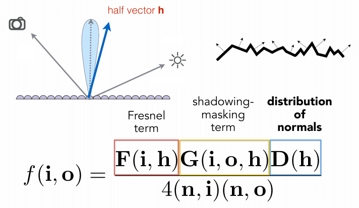
这个模型中，每个微表面都是一个完美的菲涅尔镜面。将 BRDF 用分子上三项乘积，和分母上的归一化系数表示。其中，\(n\) 是整个表面宏观上的法线方向（灰色虚线箭头）。

Normal Distribution Function¶

只有微表面的法线和 half vector \(h\) 的方向相同时，\(\omega_i\) 才能被反射到 \(\omega_o\)，所以需要计算出具有这个朝向的微表面的总面积。

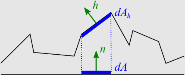
在上图中，宏观表面的面积为 \(A\)，即

\[ \int \mathrm{d}A = A \]

在上面起起伏伏的微表面中，只有 \(\mathrm{d}A_h\) 是朝向 \(h\) 的，定义法线分布函数 \(D(h)\) 满足

\[ \mathrm{d}A_h=A \cdot D(h)\mathrm{d}h \]

即

\[ D(h)= \frac{\mathrm{d}A_h}{A \cdot \mathrm{d}h} \]

因此，法线分布函数表示 \(h\) 方向上，单位立体角，单位宏观表面，朝向为 \(h\) 的微表面面积，单位是 \(sr^{-1}\)。它的归一化条件为

\[ \begin{align} 1&=\frac{1}{A}\int \mathrm{d}A\\ \\ &=\frac{1}{A} \int (n \cdot h) \mathrm{d}A_h\\ \\ &=\int_{S^2} D(h) (n \cdot h) \mathrm{d}h \end{align} \]

所以，\(D(h) (n \cdot h)\) 可以当作一个概率密度函数。上式中，\(S^2\) 表示整个球，但在图形学中使用的 \(D(h)\) 基本只在法线正半球上有值，负半球上 \(D(h)=0\)，所以积分域写成半球 \(\Omega\) 也没什么问题。

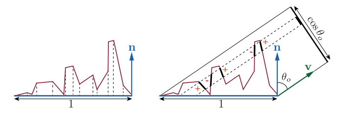
上图中，宏观表面的面积为 \(1\)，微表面的总面积就等于 \(D(h)\) 在整个球上的积分，该值是大于等于 \(1\) 的

\[ \int_{S^2} D(h) \mathrm{d}h \]

上图右侧表明，微表面和宏观表面对观察方向 \(\mathbf{v}\) 的投影面积是一样的

\[ \int_{S^2} D(h) (v \cdot h) \mathrm{d}h = v \cdot n \]

\(D(h)\) 有多种不同的模型。

Beckmann¶

\[ D(h)=\frac{\exp \left(-\dfrac{\tan^2 \theta_h}{\alpha^2} \right)}{\pi \alpha^2 \cos^4 \theta_h} \]

其中，\(\alpha\) 是表面的粗糙度，\(\theta_h\) 是 half vector \(h\) 与法线 \(n\) 的夹角。公式和正态分布比较像。

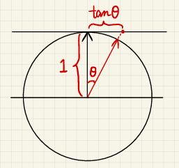
可以认为上式是定义在切空间（Slope Space）的，即以 \(\tan \theta_h\) 为自变量。将 \(\theta_h \in [0,\dfrac{\pi}{2})\) 转成 \(\tan \theta_h \in [0, +\infty)\) 后，方便套用定义在 \((-\infty,+\infty)\) 的分布（比如正态分布）。

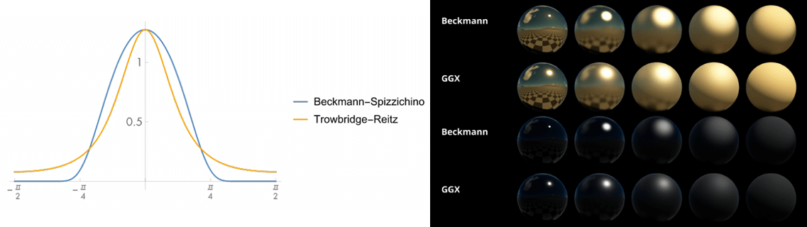
GGX (Trowbridge-Reitz)¶

\[ D(h)=\frac{\alpha^2}{\pi \left(1 + (\alpha^2-1)\cos^2 \theta_h \right)^2} \]

其中，\(\alpha\) 是表面的粗糙度，\(\theta_h\) 是 half vector \(h\) 与法线 \(n\) 的夹角。GGX 最大的特点是衰减得比 Beckmann 慢（long tail）。

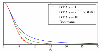
GTR (Generalized Trowbridge-Reitz)¶

\[ D(h)=\frac{k(\alpha,\gamma)}{\pi \left(1 + (\alpha^2-1)\cos^2 \theta_h \right)^2} \]

其中，\(\alpha\) 是表面的粗糙度，\(\theta_h\) 是 half vector \(h\) 与法线 \(n\) 的夹角，\(\gamma\) 用于控制尾部的形状

\[ k(\alpha,\gamma)=\begin{cases} \dfrac{(\gamma-1)(\alpha^2-1)}{1-\alpha^{2(1-\gamma)}} & \text{ where } \gamma \ne 1 \wedge \alpha \ne 1 \\ \dfrac{\alpha^2 - 1}{\ln (\alpha^2)} & \text{ where } \gamma = 1 \wedge \alpha \ne 1 \\ 1 & \text{ where } \alpha=1 \end{cases} \]

当 \(\gamma=2\) 时就是 GGX
当 \(\gamma\) 较大时，接近 Beckmann

Shadowing-Masking / Geometry Term¶

微表面可能相互遮挡，在 Grazing Angle 时，这个现象会比较明显。具体分为两种

Shadowing：光源发出的光线被遮挡

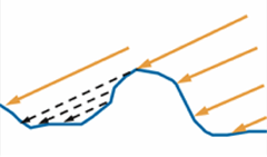
Shadowing
Masking：微表面反射的光线被遮挡

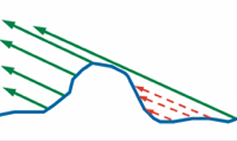
Masking

基本都用 Smith Shadowing-Masking 来计算。通常还会把该项与 BRDF 分母结合成 Visibility 项

\[ V(\mathbf{l},\mathbf{v},\mathbf{h})=\frac{G(\mathbf{l},\mathbf{v},\mathbf{h})}{4 (\mathbf{n} \cdot \mathbf{l})(\mathbf{n} \cdot \mathbf{v})} \]

其中，\(\mathbf{l}\) 是光源方向（对应入射方向 \(\mathbf{i}\)），\(\mathbf{v}\) 是视线方向（对应出射方向 \(\mathbf{o}\)）。这个分式通常能约分，减少计算量。

分离形式¶

把 Shadowing 和 Masking 当成两个不相关的事件，用 \(G_1(\mathbf{l},\mathbf{h})\) 表示 Shadowing，用 \(G_1(\mathbf{v},\mathbf{h})\) 表示 Masking

\[ G(\mathbf{l},\mathbf{v},\mathbf{h}) \approx G_1(\mathbf{l},\mathbf{h}) G_1(\mathbf{v},\mathbf{h}) \]

其中

\[ G_1(\mathbf{s},\mathbf{h})=\frac{1}{1+\Lambda(\mathbf{s})} \]

\(\Lambda(\mathbf{s})\) 和具体使用的法线分布函数（NDF）有关，GGX 对应的是

\[ \Lambda_{GGX}(\mathbf{s})=\frac{-1+\sqrt{1+\dfrac{1}{a^2}}}{2}, \quad a=\frac{1}{\alpha \tan \theta} \]

其中，\(\theta\) 是 \(\mathbf{n}\) 和 \(\mathbf{s}\) 的夹角，计算方法

\[ a^2=\frac{\cos^2 \theta}{\alpha^2 (1-\cos^2 \theta)}=\frac{(\mathbf{n} \cdot \mathbf{s})^2}{\alpha^2 (1-(\mathbf{n} \cdot \mathbf{s})^2)} \]

带入公式，最后得到

\[ V(\mathbf{l},\mathbf{v},\mathbf{h})=\frac{1}{\left((\mathbf{n} \cdot \mathbf{l})+ \sqrt{\alpha^2 + (1-\alpha^2)(\mathbf{n} \cdot \mathbf{l})^2} \right) \left((\mathbf{n} \cdot \mathbf{v})+ \sqrt{\alpha^2 + (1-\alpha^2)(\mathbf{n} \cdot \mathbf{v})^2} \right)} \]

UE5 中的实现（a2 指 \(\alpha^2\)）

// Smith term for GGX
// [Smith 1967, "Geometrical shadowing of a random rough surface"]
float Vis_Smith( float a2, float NoV, float NoL )
{
    float Vis_SmithV = NoV + sqrt( NoV * (NoV - NoV * a2) + a2 );
    float Vis_SmithL = NoL + sqrt( NoL * (NoL - NoL * a2) + a2 );
    return rcp( Vis_SmithV * Vis_SmithL );
}

Schlick 提出过一个近似算法 ²，UE 改进以后得到 ³

\[ G_1(\mathbf{s})=\frac{\mathbf{n} \cdot \mathbf{s}}{(\mathbf{n} \cdot \mathbf{s})(1-k)+k}, \quad k=\frac{\alpha}{2} \]

// Tuned to match behavior of Vis_Smith
// [Schlick 1994, "An Inexpensive BRDF Model for Physically-Based Rendering"]
float Vis_Schlick( float a2, float NoV, float NoL )
{
    float k = sqrt(a2) * 0.5;
    float Vis_SchlickV = NoV * (1 - k) + k;
    float Vis_SchlickL = NoL * (1 - k) + k;
    return 0.25 / ( Vis_SchlickV * Vis_SchlickL );
}

Multiple Bounces¶

目前还没考虑 Multiple Bounces，所以会损失能量。

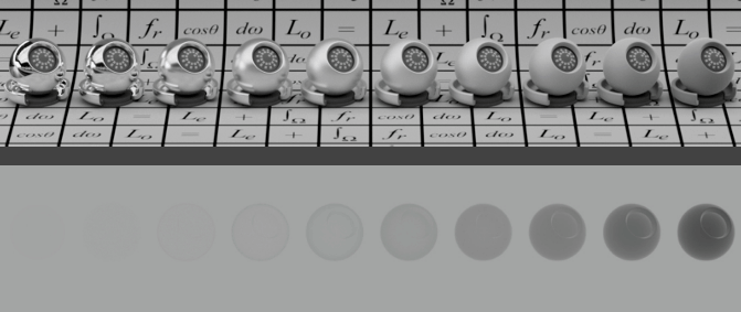
图中从左往右粗糙度变大，整体明显在变暗。

Todo

The Kulla-Conty Approximation

参考¶

Does "grazing angle" have a general definition? : r/computergraphics ↩
Schlick C. An inexpensive BRDF model for physically‐based rendering[C]//Computer graphics forum. Edinburgh, UK: Blackwell Science Ltd, 1994, 13(3): 233-246. ↩↩
Karis B, Games E. Real shading in unreal engine 4[J]. Proc. Physically Based Shading Theory Practice, 2013, 4(3): 1. ↩
Hammon E, Engineer L S, Entertainment R. Pbr diffuse lighting for ggx+ smith microsurfaces[C]//Game Dev. Conf. 2017. ↩

根据指定分布采样